Testing Protocol
- We split the data randomly into 50% Training and 50% Testing.
- We pretend that we have two competing insurance companies. One adopts the Algorithmic Approach and the other the Traditional. We refer to these companies as company A and company T respectively.
- Each company builds a claim frequency model using only the Training data and their selected modelling methodology.
- Each company then provides a quoted premium to each risk in the test set. Both companies set their quote using their respective claims frequency model. They do this by multiplying the expected number of claims by an assumed average claim size of £3,000.
- Each risk in the test set “purchases” insurance from the insurer with the lowest quote.
- Using the actual claims in the test data we assess the relative performance of each insurance company.
We repeated the above process 10 times- each time we used a different seed for the random assignment in step 1.
Performance
The table below shows the average performance across the 10 iterations.
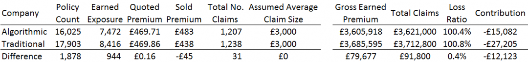
We observe the following
- The Average Quoted Premium is very close, with Company T £0.16 more expensive than Company A on average.
- However Company T won approximately 11% more business, writing 1,878 more policies than Company A.
- Company A however achieves an average sold premium almost £50 higher than Company T
- We assume an Actual Average Claim size of £3,000 across the board which is in line with both companies assumptions. Therefore any difference in financial performance is purely down to the accuracy of the respective claim frequency models
- Company A’s financial performance is much better- with a Loss Ratio improvement of 0.4% and difference in Contribution of £12,000 (both companies made a loss however due to higher overall claims frequencies)
Understanding the Performance
To understand the performance further it is useful to look at the difference in quotes from the two Companies. We define the Premium Difference = Company A Quote – Company T Quote
The table below shows the percentiles along the distribution of Premium Differences for each iteration of the test.
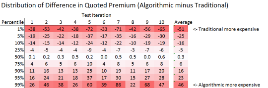
If the premium difference is positive this means that Company A was more expensive than Company T, and the risk in the test would purchase the insurance from Company T. Notice that for each iteration the median price difference was positive. This means that for each iteration, Company T was cheaper more often than Company A and therefore won more business.
It is also useful to consider the premium differences in the extremes of the distribution. Specifically we compare the premium difference at the 5% percentile to the 95% level. What we see is that in all test iterations the 5% percentile is greater in magnitude than the 95% percentile. This means that although Company T is cheaper more often, when they are expensive they are MUCH more expensive. Since these high prices do not get taken up it means that the average sold premium is much lower than the average quoted premium. It is our experience that this issue is prevalent within the insurance industry, and that the Algorithmic Pricing approach would go some way to alleviate it.
Expected Benefits
We have seen that on a relatively simple dataset with 6 rating factors a move to Algorithmic Pricing delivers a loss ratio improvement of 0.4%, a 10% improvement in average premiums and strong levels of contribution. As the pricing datasets get wider with more variables to be tested, the expected benefits will increase dramatically. Similarly we have only applied this to claims frequency- if we were to apply this to claims severity we would expect to see further improvements in performance. We therefore expect that the move to Algorithmic Pricing would deliver at least a 1% improvement in loss ratio whilst increasing average premiums and total contribution.